R Studio Download Package Already Dowloaded

LabVIEW can be used to communicate with any APT-based controller via ActiveX technology. In LabVIEW, you build a user interface, known as a front panel, with a set of tools and objects and then add code using graphical representations of functions to control the front panel objects. The LabVIEW tutorial provides some information on using ActiveX to create control GUIs for apt-driven devices within LabVIEW. The LabVIEW tab provides an overview of some basic information about using apt-based controllers in LabVIEW. The Getting Started tab explains the basic setup procedure that needs to be completed before using a LabVIEW GUI to operate an apt-based device. The Basic VIs, Intermediate VIs, and Advanced VIs tabs provide a summary of LabVIEW virtual instrument (VI) examples provided by Thorlabs to help you get started with creating programs for your controllers in LabVIEW.

A comprehensive guide to using LabVIEW with APT can be dowloaded here.

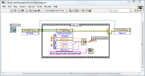
Click to Enlarge
APT Controls can be placed in the LabVIEW environment.

Typically, a Windows development system (such as LabVIEW) will allow a third-party ActiveX Control to be incorporated into the environment for ease of use by the software developer.

Adding a Thorlabs ActiveX Component to LabVIEW

1. From the Main Menu bar, select 'Controls/ActiveX/Container' to place an ActiveX Container on the front panel.
2. Right click the ActiveX container created at item (1) to display the short cut menu.
3. Select 'Insert ActiveX Object' to display the 'Select ActiveX Object' dialog box.
4. From the top menu bar, select 'Create Control'.
5. From the 'Components' list displayed, select the Thorlabs components required, (e.g., MG17Motor, MG17NanoTrak^®, MG17 Piezo, MG17Logger). Note: If a checkmark is placed in the Validate Servers checkbox, LabVIEW verifies the server and lists only the servers in the registry that actually exist on your computer. If a checkmark is not placed in the Validate Servers checkbox, LabVIEW does not verify the server and lists all servers in the registry.
6. On the block diagram, select 'Functions/Communication/ActiveX/Invoke Node'.
7. Wire the container 'refnum' to the reference input of properties and methods within the diagram.

Once the control is placed on the front panel, it can be used in the same way as any other LabVIEW control. However, each APT Control must be activated by carrying out the following two steps. For detailed instructions, see the blue box titled Creating an ActiveX Property or Method in LabVIEW.

1. The 'HWSerialNumber' property must be set to the correct (factory programmed) hardware unit serial number.
2. The 'StartCtrl' method must be called in order to activate the control.

A guide to using the APT software within a LabVIEW environment can be found here.

Note: Thread allocation in LabVIEW is dynamic. The number of threads and the usage of thread allocation will vary with each application. If the thread allocation is important in your application, some information on multithreading is provided below.

Working virtual instrument (VI) files are available with basic, intermediate, and advanced examples of how to perform general programming tasks within a LabVIEW environment (see the Basic VIs, Intermediate VIs, and Advanced VIs tabs). Useful comments have been added to the software to further explain each step in the program. These examples, which can be run with either an actual hardware configuration or a simulated configuration, interact with the hardware via the APT Server, which is downloadable from our website. Note that while the simulated server can be used, some of the more advanced alignment operations will not function as with real hardware due to the requirement for 'real' power feedback signals which are not simulated. The examples do not contain extensive information on the installation and operation of the associated hardware and should be used in conjunction with the handbooks.

If you have any questions or comments about these examples, please contact techsupport@thorlabs.com.

LabVIEW Multithreading
LabVIEW allocates several different types of threads:

• User Interface Thread: This thread is used for screen drawing, keyboard/mouse input, and certain types of VI execution, such as attribute nodes and thread-unsafe CINs and DLLs.
• Timer Threads: A pair of these threads is used internally by LabVIEW (Windows NT allocates one additional thead to be used internally).
• Execution Threads: There are twenty of these threads used per CPU in your system. LabVIEW has five "execution systems", and each execution system allocates threads for four different normal priorities. This accounts for twenty threads, not counting the user interface thread, which can also be used for execution. Execution thread allocation is based on how many processors you have in your system, so a dual processor computer will have forty execution threads plus the other threads mentioned above.

On Windows NT, threads are dynamically allocated for certain operations using the ActiveX client interface to control LabVIEW. So, for a single processor system, 23 or 24 threads are allocated when the application starts. If you are using the ActiveX client interface, more may be allocated while running your VIs.

Priorities:
Subroutine VIs always use the execution system of their caller, since staying in the same execution system is the most efficient. The "background priority" does not normally have threads allocated for it. VIs running at this priority will use the next higher priority threads when nothing else is available to run.

APT and LabVIEW Threading Issues:
APT can only be accessed by a single threaded client application. As LabVIEW is inherently multithreaded, each access to the APT software must be constrained to a single execution thread. Property Nodes cause a switch to the UI thread in the LabVIEW environment as well as other LabVIEW-based ActiveX functionality. To ensure single-threaded access to the APT software, the VI must run in the user interface thread. Currently, without enforcing your VI to run in the user interface thread, LabVIEW cannot thread marshal access to the APT software and will result in the following LabVIEW error: "Error 3006 occurred at Automation Interface Execution System."

Creating an ActiveX Property or Method in LabVIEW

A new 'Property Node' or 'Method Node" for an ActiveX object can be created directly within the block diagram without having to navigate the function palette. Property and Method Nodes can be added by using the drop down menu system within LabVIEW.

• Multiple Property Nodes and Method Nodes can be created for the same object.
• In LabVIEW, a Method Node is sometimes referred to as an Invoke Node.

To create a Property Node or Method Node for an ActiveX object:

1. Right-click the ActiveX object and select 'Create Property' or 'Create Method' from the shortcut menu. The object can be a control on the front panel within an ActiveX container, an ActiveX refnum or a terminal from another VI, a function, or a node.
2. On the block diagram, click where you want to place the Property Node or Method Node. A preoprty Node or Method Node appears on the block diagram where you clicked.
3. Right-click in the white area of the Property Node or Method Node, and select the property or method to access it.

Examples of how to create Methods in LabVIEW are provided in the videos below.

Working with ActiveX Events in LabVIEW

ActiveX events allow all of the data to be stored for a specific action that occured as a result of an ActiveX communication. The following procedure shows how to create a VI that creates and waits on an ActiveX event queue and then destroys the event queue. (Note: An event queue is a tag that corresponds to an internal list of events that an ActiveX control receives.)

1. On the block diagram, select Functions/Communication/ActiveX/ActiveX Events/Create ActiveX Event Queue.
2. Wire the ActiveX Container refnum or the ActiveX Automation refnum to the Automation RefNum input of the 'Create ActiveX Event Queue VI'.
3. Select Functions/Communication/ActiveX/ActiveX Events/Wait On ActiveX Event VI'.
4. Wire the Event Queue output from the 'Create ActiveX Event Queue VI' to the Event Queue input of the 'Wait On ActiveX Event VI'.
5. Select Functions/Communications/ActiveX/ActiveX Events/Destroy ActiveX Event Queue VI'.
6. Wire the Event Queue output from the 'Wait On ActiveX Event VI' to the Event Queue input of the 'DestroyActiveX Event Queue VI'.
7. When an event is fired, event data is returned from the Wait On ActiveX Event VI, which can be acted upon within the diagram.

Examples of how to create Properties in LabVIEW are provided in the videos below.

Tutorial Videos

Full ActiveX support is provided by LabVIEW and the series of tutorial videos below illustrates the basic building blocks in creating a custom APT motion control sequence. We start by showing how to call up the Thorlabs-supplied online help during software development. Part 2 illustrates how to create an APT ActiveX Control. ActiveX Controls provide both Methods (i.e. Functions) and Properties (i.e. Value Settings). Parts 3 and 4 show how to create and wire up both the methods and properties exposed by an ActiveX Control. Finally in Part 5 we pull everything together and show a completed LabVIEW example program that demonstrates a custom move sequence.

Disclaimer: The videos below were originally produced in Adobe Flash. Following the discontinuation of Flash after 2020, these tutorials were re-recorded for future use. The Flash Player controls still appear in the bottom of each video, but they are not functional.

Part 1: Accessing Online Help

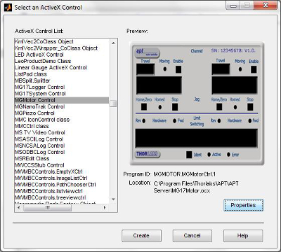
Part 2: Creating an ActiveX Control

Part 3: Create an ActiveX Method

Create an ActiveX Method (Alternative)

Part 4: Create an ActiveX Property

Create an ActiveX Property (Alternative)

Part 5: How to Start an ActiveX Control

Getting Started

The steps below outline the startup procedure for using the example virtual instruments (VIs) and connecting them to an APT-controlled device in your lab. Once you have finished this start up procedure, you can use the VIs outlined in the Basic VIs, Intermediate VIs, and Advanced VIs tabs.

1. Download the Examples from the relevant section (Basic, Intermediate, or Advanced) to the desired location on your PC.
2. Associate the Axes. To ensure that a particular stage is driven properly by the system, a number of parameters must first be set. These parameters relate to the physical characteristics of the stage being driven (e.g., min and max positions, leadscrew pitch, homing direction, etc.). To assist in setting these parameters correctly, it is possible to associate a specific stage type and axis with the motor controller channel using the APT Config utility. Once this association has been made, the APT server applies the suitable default parameter values automatically upon boot up of the software. See the APT Config Utility Helpfile for details on how to assign a stage type and axis.
3. Setting the Serial Numbers. The routines are hard coded to run the following preconfigured serial numbers:

   Motor - 20000001
   Piezo - 21000001
   NanoTrak^® - 22000001

In the APT server, the serial number must be changed accordingly in the VI diagram, whether using actual hardware or a simulated configuration. This is commented within the diagram. In the case of hardware, the serial number is on the rear of each unit.

Basic Virtual Instrument (VI) Examples

These basic examples contain all the information needed to get started using the APT Server with LabVIEW, and are not intended to be used as the basis for any custom application. The use of each ActiveX control is demonstrated in a simple .vi file, which shows how the associated ActiveX methods and properties are used. Furthermore, if an error does occur from the server, a dialog box will pop up to inform the user of the error, and the VI will stop running.

The VI's are split into five sections dependent on the control with which they are associated: Motor, NanoTrak^®, Piezo, Strain Guage, or Solenoid.

Motor VIs

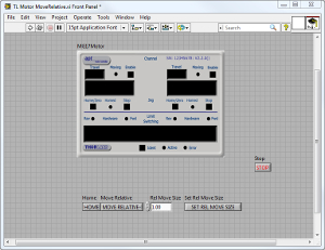
Click to Enlarge
A Screenshot of the GUI Interface of TL Motor MoveHome.vi

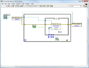
Click to Enlarge
A Screenshot of the LabVIEW Code of TL Motor MoveHome.vi

A zipped file containign all of the Motor VIs can be downloaded here.

TL Motor MoveHome.vi
This VI Moves the axis of the stage to the Home position.

Each axis on the associated stage has settings for the Zero Offset and Minimum Position parameters. The Zero Offset is the distance between the negative limit switch and the end of travel. The Minimum Position is the minimum absolute position that can be set for the stage axis. Typically, when the TL Motor MoveHome.vi is run, the stage axis moves to its negative limit and then moves forward by a set distance (zero offset). The absolute position count is then reset to zero to provide the reference point for all subsequent absolute moves. If position is lost on a stage axis, the MoveHome method should be called to re-establish the zero (Home) position.

TL Motor MoveAbsolute.vi
This VI moves the axis of the stage to the specified absolute position. The position is measured from the Home position in millimeters.

TL Motor MoveRelative.vi
This VI moves the asix of the stage a specified distance, relative to the present position.

Click to Enlarge
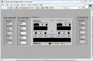
A Screenshot of  the LabVIEW Code layer of TL Motor SetGetStageAxisInfo.vi

Click to Enlarge
A Screenshot of the GUI Interface of TL Motor SetGetStageAxisInfo.vi

TL Motor SetGetStageAxisInfo.vi
This VI sets and retrieves data describing the properties of the stage, producing settings that are specific to the design of the associated stage.

• The Units parameter contains the units of measure for stage motion in either millimeters or degrees, whichever is relevant.
• The MinPos and MaxPos parameters contain the positions of the minimum and maximum travel limits respectively, and are determined by their displacement from the Home position. MinPos is usually set to zero.
• The Pitch parameter returns the pitch of the motor leadscrew in mm or degrees per rev, which is used to calculate the distance moved for each revolution of the motor.
• The DirSense parameter is for future development and is not implemented at this time.

TL Motor SetGetVelParams.vi
This VI is applicable to moves initiated from software by running the TL Motor MoveRelative.vi or TL Motor MoveAbsolute.vi. It allows the trapezoidal velocity profile parameters to be set for all moves. Parameters are set in real world units (mm or degrees) dependent upon stage type.

TL Motor MoveComplete.vi
The TL Motor MoveComplete.vi must be run with a correctly entered serial number. The MoveComplete.vi presents the user with a motor GUI panel, which can be used to move motors by pressing the job buttons or entering a position in the display. When the move is complete, the MoveComplete CallBack.vi is called and run. This second VI displays a message in the Events dialog box to state that the move has completed.

NanoTrak^® VIs

A zipped file containing all of the NanoTrak^® VIs can be downloaded here.

TL NanoTrak LatchTrack.vi
This VI sets the tracking mode for the NanoTrak. When set to Latched, scanning is disabled and the piezo drives are held at the present position. When set to Track, scanning is enabled and the NanoTrak follows the position of maximum power.

TL NanoTrak SetGetCircDia.vi
This VI sets and retrieves the diameter fo the NanoTrak scanning circle. The circle diameter is measured on a scale (NanoTrak units) such that 10 units is the width and height of the screen. If, for example, the NanoTrak is driving a 20 micron actuator, a circle diameter of 1 unit will result in a real diameter of 2 microns. The scanning circle diameter can have values in the range of 0 to 5 with a value of 5 corresponding to one half the range of piezo motion.

Note: If the NanoTrak is latched when this method is called, the circle diameter will not change. When the NanoTrak is set to Track mode, the circle diameter will change to the value set in this method.

TL NanoTrak SetGetCircDiaLUTVal.vi
This VI enables a look up table (LUT) of circle diameter values (in NanoTrak units) to be specified as a function of input range. The system then uses the values in this LUT to modify circle diameter in relation to the input range currently selected. This mode of adjustment allows the appropriate circle diameters to be applied on an application-specific basis.

TL NanoTrak SetGetCircleHomePos.vi
This VI sets and retrieves the circle home position. The present horizontal and vertical coordinates of the home position are displayed in the 'Initial Pos' field. Both position outputs can have values in the range of 0.0 to 10.0 (NanoTrak units), with (5.0, 5.0) representing the display's origin (screen center).

TL NanoTrak SetGetLoopGain.vi
This VI sets and retrieves the feedback loop gain. The gain setting is used to ensure that the DC level of the input (feedback loop) signal lies within the dynamic range of the input.The present gain value is displayed in the 'Initial Gain' field. The gain can be changed by entering a value (in the range 100 to 10,000) in the 'New Gain' field.

TL NanoTrak SetGetPhaseComp.vi
This VI sets and retrieves the phase compensation for the horizontal and vertical components of the circle path.

The feedback loop scenario in a typical NanoTrak application can involve the operation of various electronic and electromechanical components (e.g., power meters and piezo actuators) that could introduce phase shifts around the loop and thereby affect tracking efficiency and stability. These phase shifts can be cancelled by setting the 'Phase Compensation' factors. This VI sets and retrieves the phase compensation for the horizontal and vertical components of the circle path.

The present values are displayed in the 'Initial Phase Comp' field. These values can be changed by entering different values into the 'New Phase Comp' field. The values are specified in degrees and lie in the range -180.0 to 180.0 degrees.Typically, both phase offsets will be set the same, although some electromechanical systems may exhibit different phase lags in the different components of travel and so require different values.

TL NanoTrak SetGetRangingMode.vi
This VI sets and retrieves the ranging mode. The ranging mode currently selected is displayed in the first box of the 'Initial Ranging Mode' field. It can be set by entering a number 1 through 4:

1. Changes the ranging mode to to Auto ranging at the range currently selected.
2. Changes the ranging mode to Manual ranging at the range currently selected.
3. Changes the ranging mode to manual ranging at the range set in the SetRange method (or the 'Settings' panel). When auto-ranging mode is selected, range changes occur whenever the relative input power signal reaches the upper or lower end of the currently set range.
4. Changes the ranging mode to Auto ranging at the range set in the SetRange method (or the 'Settings' panel). When auto-ranging mode is selected, range changes occur whenever the relative input power signal reaches the upper or lower end of the currently set range.

The second box of the 'Initial Ranging Mode' field specifies how these range changes are implemented by the system:

1. The unit visits all ranges when ranging between two input signal levels.
2. Only odd numbered ranges between the two input signals will be visited.
3. Only even numbered ranges between the two input signal levels will be visited. These latter two modes are useful when large rapid input signal fluctuations are anticipated. This is because the number of ranges visited is halved to give a more rapid resonse.

The ranging mode can be changed by entering different values into the 'New Ranging Mode' field.

Piezo VIs

A zipped file containing all of the Piezo VIs can be downloaded here.

TL Piezo GetMaxTravel.vi
In the case of actuators with built-in position sensing, the Piezoelectric Control Unit can detect the range of travel of the actuator since this information is programmed in the electronic circuit inside the actuator. This VI retrieves the maximum travel for the piezo actuator associated with the channel specified by the lChanID parameter, and returns a value (in microns) in the plMaxTravel parameter.

TL Piezo SetGetControlMode.vi
When in closed-loop mode, position is maintained by a feedback signal from the piezo actuator. This is only possible when using actuators equipped with position sensing. This VI sets the control loop status. For more details, please refer to the APT server help file (After APT installation, this can be found in Start/All Programs/Thorlabs/APT/Help).

TL Piezo SetGetPosOutput.vi
This VI sets and retrieves the position of the piezo actuator.

The current position of the actuator is displayed in the 'Initial Position' field. The position of the actuator is relative to the datum set for the arrangement using the ZeroPosition method. Once set, the extension of the actuator will be read and scaled automatically to a position in microns, for whichever actuator is connected to the control module. Note: The SetPosOutput VI is applicable only to actuators equipped with position sensing and operating in closed loop mode. Actuators fitted with feedback circuitry can be interrogated by the Piezo module for maximum travel in microns (see the GetMaxTravel.vi).

The position of the actuator can be changed by entering a different value in the 'New Position' field.

TL Piezo SetOutputLUTValue.vi
It is possible to use the controller in an arbitrary Waveform Generator Mode (WGM). Rather than the unit outputting an adjustable but static voltage or position, the WGM allows the user to define a voltage or position sequence to be output, either periodically or a fixed number of times, with a selectable interval between adjacent samples. This waveform generation function is particularly useful for operations such as scanning over a particular area, or in any other application that requires a predefined movement sequence.

The waveform is stored as values in an array, with a maximum of 8000 samples per channel which represent either voltage or position. If open loop operation is specified when the samples are output, then their meaning is voltage; if the channel is set to closed loop operation, the samples are interpreted as position values. If the waveform to be output requires less than 8000 samples, it is sufficient to download the desired number of samples.

Strain Guage VI

A zipped file containing the Strain Guage VI can be downloaded here.

TL Strain Guage Reader GetReading.vi
This VI returns the current reading of the strain gauge associated with the Strain Gauge Reader.

The units applicable are dependent on the current operating mode. If the unit is operating in Position mode, then the vi returns a position value in microns. If the unit is in Voltage mode, then the vi returns a Voltage. If the controller is in 'Force Sensing Mode' then a force value in Newtons is returned. The returned data values are sampled at 500 Hz, which is particularly useful in touch probe or force sensing applications where rapid polling of the force reading is important.

All values are relative to the datum set for the arrangement.

Solenoid VI

A zipped file containing the Solenoid VI can be downloaded here.

TL SetOperatingMode.vi
This VI sets the operating mode of the Solenoid Controller unit. For more details, please refer to the APT server help file (After APT installation, this can be found in Start/All Programs/Thorlabs/APT/Help).

Intermediate Virtual Instrument (VI) Examples

The Intermediate Examples contain five routines, written using the APT Server. These are only intended to be used as examples when writing custom applications, and all parameters are hard coded. Before the examples can be used as the basis for any custom application development, parameters may need to be changed. For example, the scan routines may require different start point and interval values. The threshold for the power range to locate during a search may also be different. If an error occurs from the server, a dialog box will pop up to inform the user of the error, and the VI will stop running.

The function of each VI is explained briefly below. The files can be downloaded here.

2D Raster Scan Pattern

Motor2DScan.vi
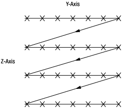
This VI shows a basic two-dimensional raster scan using a motor control, which is the most basic scan pattern. Coordinates are generated along the Y axis between a lower and upper search limit. Once the upper limit is reached, the search is stepped in the Z axis and begins again. The number of coordinates generated is dependent upon the search area and the step size.

MotorScan2DFindRange.vi
This VI is an extension of the Motor 2D scan. A NanoTrak^® control is included, and the scan is exited when the signal being searched exceeds a predefined threshold value.

Piezo2DScan.vi
This VI shows a basic two-dimensional raster scan using a piezo control.

This is the most basic scan pattern. Coordinates are generated along the Y axis between a lower and upper search limit. Once the upper limit is reached, the search is stepped in the Z axis and begins again. The number of coordinates generated is dependent upon the search area and the step size.

PiezoNanoTrak2DScanFindRange.vi
This VI is an extension of the Piezo 2D scan. A NanoTrak control is included, and the scan is exited when the signal being searched exceeds a predefined threshold value.

MotorNanoTrak2DRevector.vi
In any application, when the NanoTrak is set to tracking mode, the NanoTrak is limited to the range of the piezos in order to track the signal. If, due to thermal drift or other external influences, the NanoTrak reaches the edge of its screen it will lose the signal due to the range of the piezos. A revector routine checks the circle position, and if the circle position is not near the center of the NanoTrak's screen, motors are used to ensure that the NanoTrak has sufficient range to continue tracking the signal.

Advanced Virtual Instrument (VI) Examples

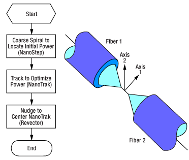
The Thorlabs approach to alignment is based on a combination of stepper motors (NanoSteps) and piezo positioners. The stepper motors provide coarser motion over longer range whereas the piezos provide extremely fine motion over shorter range. The piezos are driven from the NanoTrak^®, an analog instrument that optimizes the piezo extension for maximum optical power.

The Advanced Examples contain five routines, written using the APT Server. These VIs are intended to be used as examples when writing custom applications. Before the examples can be used as the basis for any custom application development, some alteration of the code may be necessary. For example, the order and process in which optimization occurs may need altering. Furthermore, if an error occurs from the server, a dialog box will pop up to inform the user of the error, and the VI will stop running. In an end application more complex error handling may be needed.The function of each VI is explained below. A zipped folder containing all of the advanced example VIs can be downloaded here.

Note: These VIs contain sample code to illustrate optimization of alignment along several sets of axes. The code may be copied and pasted into another program, but more advanced error handling must be added before this example can be run as part of an end application.

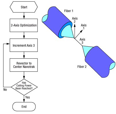
2-Axis Optimization

This virtual instrument optimizes the alignment of two parts of a system along 2 axes (for example, the alignment of two fiber tips to maximize the amount of light that is coupled from one to the other). A 2D spiral search is performed by the NanoStep motors to locate the initial (threshold) power; then the optimum power is located using the piezos, with revectoring as required. The procedure is outlined in the flow chart to the right.

A zipped folder containing all of the advanced example VIs can be downloaded here.

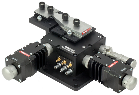
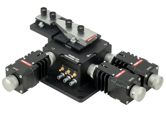
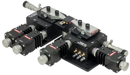
Setting Up the NanoMax Stage
For this example, we will set up a NanoMax Stage with two V-groove fiber holders as shown in the drawing below. The mechanical components are listed in the table to the right. The components that need alignment have been left out of the setup, since these will be user dependent. Connect the NanoMax stage to the PC as detailed in the handbook for your device.

Click to Enlarge
A NanoMax stage set up for the 2-Axis Optomization VI. A complete list of item #'s is provided in the table to the right.

Item #	Description	Quantity
MAX301 or MAX302	NanoMax-HS 3-Axis Stage	1
DRV001	NanoStep Actuator	2
DRV3	Differential Micrometer	1
AMA007 or AMA009	Fixed World Bracket	1
HFV001	Standard V-Groove Fiber Holdera	1
HFV002	Tapered V-Groove Fiber Holdera	1
HFC005	Standard Fiber Chuck	1
BNT001/IR	APT NanoTrak® Controller	1
BSC202	APT Stepper Motor Controller	1

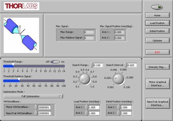
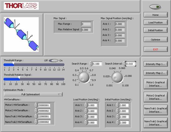
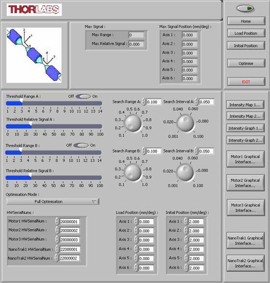
2-Axis Optimization GUI
The 2-axis optimization VI GUI is shown to the right and a description of each field is provided in the table underneath. Instructions for running the GUI are as follows:

1. Ensure your system is set up according to the instructions given on the Getting Started tab.
2. Power up the equipment.
3. Open LabVIEW and run the 2AxisOptimization.vi file.
4. Enter the serial numbers of the Stepper Motor and NanoTrak unit in your system.
5. Enter values for the Threshold Range and Threshold Relative Signal applicable to your application, then check the Threshold box.
6. Enter values for the Search Range and Search Interval applicable to your application.
7. Enter values for the Load Position and Initial Position (the default values should be satisfactory for most applications).
8. Click the button to start communication between the software and the hardware.
9. Click the Home button then wait for the motors to complete the homing movement.
10. Click the Load Position button then wait for the motors to move to the load position.
11. Load the devices to be aligned.
12. Click the Initial Position button then wait for the motors to move to the initial position.
13. Select the desired Optimization Mode and click the Optimize button to start the optimization sequence.
14. If a power threshold is not located, adjust the Threshold Range and Threshold Relative Signal to a lower setting.

General Notes:

• During the alignment, the maximum signal level located and its associated position, are displayed in the Max Signal and Max Signal Position fields.
• After the alignment sequence is completed, the NanoTrak is set to `latch' mode.
• If a large value is set in the Search Range field, and/or a small value is set in the Search Interval field, it may take a long time to generate the scan coordinates. The actual time taken to generate the coordinates is dependent upon PC performance.

Field Name	Description
Max Signal	Displays the maximum power located during the search. The power is displayed as a relative signal and a range value.
Max Signal Position	Displays the position at which the maximum power was located.
Threshold Range and Relative Signal	The combination of these two settings determines the power level to be located by the spiral search. The search is terminated when the threshold level is exceeded. The level set should be higher than the noise floor to ensure the NanoTrak® does not track to a false power peak.
Search Range and Interval	The range and interval (step size) of the search pattern (in mm).
Optimization Mode	The type of optimization to perform. Select from:	Full Optimization: A complete optimization including NanoTrak scan for max power.
		Stop Optimization Upon Threshold Signal: The optimization is stopped once the level of power found exceeds the threshold level set for the 2D scan. If no threshold level is set, a full 2D scan is performed. The system then moves to the position where max power was located.
HWSerialNums	Enter the serial numbers of each APT unit in the system.
Load Position	Moves all the motors to the initial position. These are the safe positions where load or unload operations can be performed. The positions are measured in mm (or degrees) from the Home position.
Initial Position	The position of the motors immediately prior to the commencement of an optimization. The position is measured in mm (or degrees) from the Home position.
Home	Moves all motors to the Home position.
Load Position	Moves all motors to the initial position.
Optimize	Start button for the optimization.
Exit	Stops the current LabVIEW VI. To restart a VI, select 'Run' from the LabVIEW environment.
Intensity Map	Displays a graphical representation of the search results.
Motor Graphical Interface	Displays the GUI panel for the stepper motor controller unit whose serial number is selected in the HWSerialNums field.
NanoTrak® Graphical Interface	Displays the GUI panel for the NanoTrak unit whose serial number is selected in the HWSerialNums field.

3-Axis Optimization

This VI is used to optimize the alignment of 3 axes in a system. First, a 2D spiral search is performed by the NanoStep motors to locate the initial (threshold) power. Next, the optimum power is located using the piezos, with revectoring as required. Once max power is located in axes 1 and 2, the power is further optimized by adjusting the position in axis 3, while the position in axes 1 and 2 are maintained by `nudging' the NanoTrak. The alignment is complete when a specified ceiling power is achieved.

A zipped folder containing all of the advanced example VIs can be downloaded here.

Setting Up the NanoMax Stage
For this example, we will set up a NanoMax Stage with two V-groove fiber holders as shown in the drawing below. The mechanical components are listed in the table to the right. The components that need alignment have been left out of the setup, since these will be user dependent. Connect the NanoMax stage to the PC as detailed in the handbook for your device.

Click to Enlarge
A NanoMax stage set up for the 3-Axis Optomization VI. A complete list of item #'s is provided in the table to the right.

Item #	Description	Quantity
MAX301 or MAX302	NanoMax-HS 3-Axis Stage	1
DRV001	NanoStep Actuator	3
AMA007 or AMA009	Fixed World Bracket	1
HFV001	Standard V-Groove Fiber Holdera	1
HFV002	Tapered V-Groove Fiber Holdera	1
HFC005	Standard Fiber Chuck	1
BNT001/IR	APT NanoTrak® Controller	1
BSC202	APT Stepper Motor Controller	1

3-Axis Optimization GUI
The 3-axis optimization VI GUI is shown to the right and a description of each field is provided in the table underneath. Instructions for running the GUI are as follows:

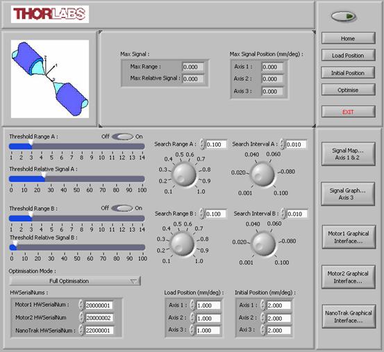
1. Ensure your system is set up according to the instructions given on the Getting Started tab.
2. Power up the equipment.
3. Open LabVIEW and run the 2AxisOptimization.vi file.
4. Enter the serial numbers of the Stepper Motor and NanoTrak unit in your system.
5. Enter values for the Threshold Range A and Threshold Relative Signal A applicable to your application, then check the Threshold box.
6. Enter values for the Search Range A and Search Interval A applicable to your application.
7. Enter values for the Threshold Range B and Threshold Relative Signal B applicable to your application, then check the Threshold box.
8. Enter values for the Search Range B and Search Interval B applicable to your application.
9. Enter values for the Load Position and Initial Position (the default values should be satisfactory for most applications).
10. Click the button to start communication between the software and the hardware.
11. Click the Home button then wait for the motors to complete the homing movement.
12. Click the Load Position button then wait for the motors to move to the load position.
13. Load the devices to be aligned.
14. Click the Initial Position button then wait for the motors to move to the initial position.
15. Select the desired Optimization Mode and click the Optimize button to start the optimization sequence.
16. If a power threshold is not located, adjust the Threshold Range A and Threshold Relative Signal A to a lower setting.

General Notes:

• During the alignment, the maximum signal level located and its associated position, are displayed in the Max Signal and Max Signal Position fields.
• After the alignment sequence is completed, the NanoTrak is set to `latch' mode.
• If a large value is set in the Search Range field, and/or a small value is set in the Search Interval field, it may take a long time to generate the scan coordinates. The actual time taken to generate the coordinates is dependent upon PC performance.

Field Name	Description
Max Signal	Displays the maximum power located during the search. The power is displayed as a relative signal and a range value.
Max Signal Position	Displays the position at which the maximum power was located.
Threshold Range A and Relative Signal A	The combination of these two settings determines the signal level to be located by the spiral search on axes 1 and 2. The search is terminated when the threshold level is exceeded. The signal level set should be higher than the noise floor to ensure the NanoTrak® does not track to a false power peak.
Search Range A and Interval A	The range and interval (step size) of the search pattern (in mm).
Threshold Range B and Relative Signal B	The combination of these two settings determines the signal level to be located by the step search on axis 3. The search is terminated when the threshold level is exceeded. The signal level set should be higher than that set for search A and less than or equal to the maximum signal level expected for the application.
Search Range B and Interval B	The range and interval (step size) of the step search (in mm).
Optimization Mode	The type of optimization to perform. Select from:	Full Optimization: A complete optimization including NanoTrak scan for max power.
		Stop Optimization Upon Threshold Signal: The optimization is stopped once the level of power found exceeds the threshold level set for the 2D scan. If no threshold level is set, a full 2D scan is performed. The system then moves to the position where max power was located.
HWSerialNums	Enter the serial numbers of each APT unit in the system.
Load Position	Moves all the motors to the initial position. These are the safe positions where load or unload operations can be performed. The positions are measured in mm (or degrees) from the Home position.
Initial Position	The position of the motors immediately prior to the commencement of an optimization. The position is measured in mm (or degrees) from the Home position.
Home	Moves all motors to the Home position.
Load Position	Moves all motors to the initial position.
Optimize	Start button for the optimization.
Exit	Stops the current LabVIEW VI. To restart a VI, select 'Run' from the LabVIEW environment.
Intensity Map	Displays a graphical representation of the search results.
Motor Graphical Interface	Displays the GUI panel for the stepper motor controller unit whose serial number is selected in the HWSerialNums field.
NanoTrak® Graphical Interface	Displays the GUI panel for the NanoTrak unit whose serial number is selected in the HWSerialNums field.

4-Axis Optimization

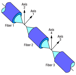
This VI is useful for aligning two NanoMax stages, each along two axes. The figure to the right shows the breakdown of where each axes is located. 2D spiral search is performed on axes 1 and 2, and on axes 3 and 4, by the NanoStep motors. Once the initial (threshold) power is located, the power is optimized using the piezos, with revectoring as required. The tracking is performed simultaneously on 2 NanoTraks (set to different frequencies), one at each end of the device being aligned.

A zipped folder containing all of the advanced example VIs can be downloaded here.

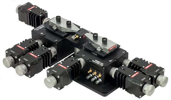
Setting Up the NanoMax Stage
For this example, we will set up a NanoMax Stage with two V-groove fiber holders as shown in the drawing below. The mechanical components are listed in the table to the right. The components that need alignment have been left out of the setup, since these will be user dependent. Connect the NanoMax stage to the PC as detailed in the handbook for your device.

Click to Enlarge
NanoMax stages set up for the 4-Axis Optomization VI. A complete list of item #'s is provided in the table to the right.

Item #	Description	Quantity
MAX301 or MAX302	NanoMax-HS 3-Axis Stage	2
DRV001	NanoStep Actuator	4
DRV3	Differential Micrometer	2
AMA029C	Fixed Platform	1
HWV001	Waveguide Mount with Vacuum Holddowna	1
HFV002	Tapered V-Groove Fiber Holdera	1
BNT001/IR	APT NanoTrak® Controller	2
BSC202	APT Stepper Motor Controller	2

4-Axis Optimization GUI
The 4-axis optimization VI GUI is shown to the right and a description of each field is provided in the table underneath. Instructions for running the GUI are as follows:

1. Ensure that your system is set up according to the instructions on the Getting Started tab.
2. Power up the equipment.
3. Open LabVIEW and run the file 4AxisOptimization.vi.
4. Enter the serial numbers of the Stepper Motor and NanoTrak unit in your system.
5. Enter values for the Threshold Range and Threshold Relative Signal applicable to your application, then check the Threshold box.
6. Enter values for the Search Range and Search Interval applicable to your application.
7. Enter values for the Load Position and Initial Position (the default values should be satisfactory for most applications).
8. Click the button to start communication between the software and the hardware.
9. Click the Home button then wait for the motors to complete the homing movement.
10. Click the Load Position button then wait for the motors to move to the load position.
11. Load the devices to be aligned.
12. Click the Initial Position button then wait for the motors to move to the initial position.
13. Select the desired Optimization Mode and click the Optimize button to start the optimization sequence.
14. If a power threshold is not located, adjust the Threshold Range and Threshold Relative Signal to a lower setting.

General Notes:

• During the alignment, the maximum signal level located and its associated position, are displayed in the Max Signal and Max Signal Position fields.
• After the alignment sequence is completed, the NanoTrak is set to `latch' mode.
• If a large value is set in the Search Range field, and/or a small value is set in the Search Interval field, it may take a long time to generate the scan coordinates. The actual time taken to generate the coordinates is dependent upon PC performance.

Field Name	Description
Max Signal	Displays the maximum power located during the search. The power is displayed as a relative signal and a range value.
Max Signal Position	Displays the position at which the maximum power was located along each axis.
Threshold Range and Relative Signal	The combination of these two settings determines the signal level to be located by the spiral search on axes 1 and 2. The search is terminated when the threshold level is exceeded. The signal level set should be higher than the noise floor to ensure the NanoTrak® does not track to a false power peak.
Search Range and Interval	The range and interval (step size) of the search pattern (in mm).
Optimization Mode	The type of optimization to perform. Select from:	Full Optimization: A complete optimization including NanoTrak scan for max power.
		Stop Optimization Upon Threshold Signal: The optimization is stopped once the level of power found exceeds the threshold level set for the 2D scan. If no threshold level is set, a full 2D scan is performed. The system then moves to the position where max power was located.
HWSerialNums	Enter the serial numbers of each APT unit in the system.
Load Position	Moves all the motors to the initial position. These are the safe positions where load or unload operations can be performed. The positions are measured in mm (or degrees) from the Home position.
Initial Position	The position of the motors immediately prior to the commencement of an optimization. The position is measured in mm (or degrees) from the Home position.
Home	Moves all motors to the Home position.
Load Position	Moves all motors to the initial position.
Optimize	Start button for the optimization.
Exit	Stops the current LabVIEW VI. To restart a VI, select 'Run' from the LabVIEW environment.
Intensity Map	Displays a graphical representation of the search results.
Motor Graphical Interface	Displays the GUI panel for the stepper motor controller unit whose serial number is selected in the HWSerialNums field.
NanoTrak® Graphical Interface	Displays the GUI panel for the NanoTrak unit whose serial number is selected in the HWSerialNums field.

6-Axis Optimization

This VI is useful for aligning two NanoMax stages, along 3 axes each, to a component in the middle. A 2D spiral search is performed on axis 1 and 2 and on axis 3 and 4 simultaneously. The NanoStep motors locate the initial (threshold) power; then the optimum power is located using the piezos, with revectoring as required. Once max power is located in axes 1, 2, 3, and 4, the power is further optimized by positioning in axis 5 and 6, while the positions along axes 1, 2, 3, and 4 are maintained by 'nudging' the NanoTrak.

The tracking is performed simultaneously on 2 NanoTraks (set to different frequencies), one at each end of the device being aligned. Similarly the nudging is performed on 4 axes to centre the circle on both NanoTraks. The alignment is complete when the specified ceiling power is achieved.

A zipped folder containing all of the advanced example VIs can be downloaded here.

Setting Up the NanoMax Stage
For this example, we will set up a NanoMax Stage with two V-groove fiber holders as shown in the drawing below. The mechanical components are listed in the table to the right. The components that need alignment have been left out of the setup, since these will be user dependent. Connect the NanoMax stage to the PC as detailed in the handbook for your device.

Click to Enlarge
NanoMax stages set up for the 6-Axis Optomization VI. A complete list of item #'s is provided in the table to the right.

Item #	Description	Quantity
MAX301 or MAX302	NanoMax-HS 3-Axis Stage	2
DRV001	NanoStep Actuator	6
AMA029C	Fixed Platform	1
HWV001	Waveguide with Vacuum Holddowna	1
HFV002	Tapered V-Groove Fiber Holdera	2
HFC005	Standard Fiber Chuck	1
BNT001/IR	APT NanoTrak® Controller	2
BSC202	APT Stepper Motor Controller	2

6-Axis Optimization GUI
The 6-axis optimization VI GUI is shown to the right and a description of each field is provided in the table underneath. Instructions for running the GUI are as follows:

1. Ensure your system is set up according to the instructions given on the Getting Started tab.
2. Power up the equipment.
3. Open LabVIEW and run the 6AxisOptimization.vi file.
4. Enter the serial numbers of the Stepper Motor and NanoTrak unit in your system.
5. Enter values for the Threshold Range A and Threshold Relative Signal A applicable to your application, then check the Threshold box.
6. Enter values for the Search Range A and Search Interval A applicable to your application.
7. Enter values for the Threshold Range B and Threshold Relative Signal B applicable to your application, then check the Threshold box.
8. Enter values for the Search Range B and Search Interval B applicable to your application.
9. Enter values for the Load Position and Initial Position (the default values should be satisfactory for most applications).
10. Click the button to start communication between the software and the hardware.
11. Click the Home button then wait for the motors to complete the homing movement.
12. Click the Load Position button then wait for the motors to move to the load position.
13. Load the devices to be aligned.
14. Click the Initial Position button then wait for the motors to move to the initial position.
15. Select the desired Optimization Mode and click the Optimize button to start the optimization sequence.
16. If a power threshold is not located, adjust the Threshold Range A and Threshold Relative Signal A to a lower setting.

General Notes:

• During the alignment, the maximum signal level located and its associated position, are displayed in the Max Signal and Max Signal Position fields.
• After the alignment sequence is completed, the NanoTrak is set to `latch' mode.
• If a large value is set in the Search Range field, and/or a small value is set in the Search Interval field, it may take a long time to generate the scan coordinates. The actual time taken to generate the coordinates is dependent upon PC performance.

Field Name	Description
Max Signal	Displays the maximum power located during the search. The power is displayed as a relative signal and a range value.
Max Signal Position	Displays the position at which the maximum power was located.
Threshold Range A and Relative Signal A	The combination of these two settings determines the signal level to be located by the spiral search on axes 1 and 2. The search is terminated when the threshold level is exceeded. The signal level set should be higher than the noise floor to ensure the NanoTrak® does not track to a false power peak.
Search Range A and Interval A	The range and interval (step size) of the search pattern (in mm).
Threshold Range B and Relative Signal B	The combination of these two settings determines the signal level to be located by the step search on axis 3. The search is terminated when the threshold level is exceeded. The signal level set should be higher than that set for search A and less than or equal to the maximum signal level expected for the application.
Search Range B and Interval B	The range and interval (step size) of the step search (in mm).
Optimization Mode	The type of optimization to perform. Select from:	Full Optimization: A complete optimization including NanoTrak scan for max power.
		Stop Optimization Upon Threshold Signal: The optimization is stopped once the level of power found exceeds the threshold level set for the 2D scan. If no threshold level is set, a full 2D scan is performed. The system then moves to the position where max power was located.
HWSerialNums	Enter the serial numbers of each APT unit in the system.
Load Position	Moves all the motors to the initial position. These are the safe positions where load or unload operations can be performed. The positions are measured in mm (or degrees) from the Home position.
Initial Position	The position of the motors immediately prior to the commencement of an optimization. The position is measured in mm (or degrees) from the Home position.
Home	Moves all motors to the Home position.
Load Position	Moves all motors to the initial position.
Optimize	Start button for the optimization.
Exit	Stops the current LabVIEW VI. To restart a VI, select 'Run' from the LabVIEW environment.
Intensity Map	Displays a graphical representation of the search results.
Motor Graphical Interface	Displays the GUI panel for the stepper motor controller unit whose serial number is selected in the HWSerialNums field.
NanoTrak® Graphical Interface	Displays the GUI panel for the NanoTrak unit whose serial number is selected in the HWSerialNums field.

Accessing an ActiveX Control in MATLAB

The APT System Software is implemented as a set of ActiveX controls that are added to the host PC control library when the APT Software is installed. These ActiveX controls typically have a user interface, which can be interacted with using one of several programming environments. The ability to use the controls within multiple programming environments is facilitated through the Microsoft^® Component Object Model (COM), which is a binary-interface standard for implementing objects that can be used in an environment different from the one in which they are created; i.e., it allows objects to be reused without knowledge of their internal implementation. A Microsoft ActiveX control is a type of in-process COM server that requires a control container, which is an application capable of hosting ActiveX controls. Programming environments and languages such as MATLAB^®, Visual C++, and C# can be used to create these control containers, thus allowing users to interact with the ActiveX controls for their own applications.

MATLAB^®
A MATLAB figure window or a Simulink^® model are types of control containers. In a typical scenario, MATLAB creates ActiveX controls in figure windows, which are manipulated by MATLAB through the controls' properties, methods, and events. In this case, Thorlabs' APT ActiveX control is used as the server and MATLAB is used as the client. Graphical user interface (GUI) components are implemented as APT ActiveX controls. By creating an ActiveX object, MATLAB can control the hardware using the APT GUI components. For more details on using MATLAB and ActiveX controls with Thorlabs' APT positioners, click here.

Visual C++
Simply create a new C++ project for your application, display the main application dialog box, and select the required APT ActiveX controls from the library displayed. For more information, the videos below demonstrate how to get an APT ActiveX control running within Visual C++ and how to program a custom positioning sequence.

APT Programming with Visual C++ Part 1

APT Programming with Visual C++ Part 2

C#
Examples are available that contain sample programs to get started using the APT Server with C#. The use of each ActiveX control is demonstrated in an example project file, which can be opened in Visual Studio or another similar development package. The examples are split into four sections dependent on the control with which they are associated: Motor, NanoTrack^®, Piezo, and Quad Detector. Examples can be downloaded here.

Posted by: brown121.blogspot.com

Source: https://www.thorlabs.com/newgrouppage9.cfm?objectgroup_id=8348